Essentials of Microcontroller Use Learning about Peripherals: 5 of 6
In our previous four sessions, we did some programming that made use of the MCU's peripheral functions. As we've explained, MCUs come with built-in peripheral capabilities that allow them to respond easily to a broad range of relatively standard requirements. But of course, MCUs and peripherals won't do anything at all until you write programs for them. In this two-part session, we will look at the relationship between programs and the MCU.
About MCU Memory
In this series, we have already written a number of programs to run on the RX63N MCU mounted on the GR-SAKURA board. As you remember, we used our online compiler to convert the source code into object code, and then we loaded the object code into the MCU in much the same way we would store the code into a USB stick. So where exactly is this code stored within the MCU, and how does it get executed? Let's answer these questions as we look at the relationship between the MCU and the programs that run on it.
Main Memory vs. External Memory
Memory is used to store both program code and data. Memory within the CPU has a different role than memory outside the CPU, as follows.
Main Memory
The CPU can access main memory rapidly and directly. This memory stores the program code and data for currently executing programs.
External Memory
Also referred to as secondary memory. Holds program code and data for programs that are not currently executing. Not directly accessible by the CPU. For example, may be accessed via USB, Serial or Parallel I/O.
To run a program stored in external memory, the MCU must first load the code into the main memory.
You are probably aware that main memory comes in two types: ROM (read only memory, with fixed content) and RAM (random access memory, with writable content). However, please note that the difference between ROM and RAM is not relevant to the present discussion, since both are part of the main memory and serve the same functional purpose. (For more about ROM and RAM, feel free to review the Introduction to Microcontrollers - Part 1.
Address Space (Memory Space)
The address space (also called memory space) is the entire range of memory that can be directly accessed by the MCU. It covers all of main memory. Locations within this space are identified by address: each byte of memory has its own address. Address values are typically written in hexadecimal notation.
Some CPUs use 4-bit addresses (4 hexadecimal digit), others use 8 bits, 16 bits, 32 bits, and so on. The RX63N on the GR-SAKURA is a "32-bit MCU." Each address consists of 32 hexadecimal digits; this gives a total of 232 addressable bytes. The address space, therefore, is 4,294,967,296 bytes (4×1024×1024×1024), a size that is also referred to as 4 gigabytes ("4 GB"; see Column 1). Large address spaces allow for high-capacity memories that can store very large programs—allowing for effective loading and use of powerful and sophisticated applications.
Figure 1 shows the 4 GB address space of a 32-bit CPU. Address values, as indicated above, are written in hexadecimal notation (see Column 2). Each row holds four addressable bytes; the number at the left of the row is the address of the leftmost byte. That's why the numbers running down the left are in increments of four.
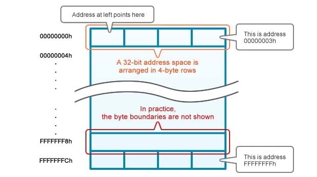
Figure 1. Address Space Representation
Column 1: Bits, Bytes, MB, GB, TB
In computing, the smallest data unit is a bit(from "Binary digit"), which takes one of two values, typically represented as 0 and 1. Bits are usually addressed and handled in groups of eight; such a group is called a byte. So three bytes, for example, consists of 24 bits. (Note also that the abbreviation for "bit" is a lowercase, "b", while the abbreviation for byte is an uppercase "B".)
Memory capacity is expressed in multiples of bytes. The most common units are KB (kilobytes), MB (megabytes), GB (gigabytes), and TB (terabytes). These names derive from the prefixes kilo (thousand), mega (million), giga (billion), and tera (trillion). It is often the case, therefore, that a term such as 1GB will be used to mean 1000MB. But in the computer world, powers of two reign supreme, and in most cases (although not all) these units have the following values.
- 1KB = 210bytes = 1,024 bytes
- 1MB = 1,024KB = 220 = 1,048,576 bytes
- 1GB = 1,024MB = 230 = 1,073,741,824 bytes
- 1TB = 1,024GB = 240 = 1,099,511,627,776 bytes
Column 2: Hexadecimal Address Notation
Addresses are generally expressed as hexadecimal values. Consider a 16-bit address space, with a total of 216 addresses. In decimal notation, these addresses would run 0, 1, 2 … 9, 10, 11 … 65535. In hex notation, however, the addresses run: 0h, 1h … 9h, Ah, Bh … Fh, 10h, 11h … FFFFh. Note that where decimal notation uses ten numerals (0 to 9), hexadecimal requires 16, (0 … 9, A … F). Notice also that A (hex) is equal to 10 (decimal), and F (hex) is equal to 15 (decimal). In general, an "h" suffix is appended to hex values for clarity: so, for example, 11h = 17 (decimal).
![]()
Where Is the Program Code Stored? (Vector Tables)
When the CPU starts to run a program, it must read the first instruction from memory. But what memory address should it go to for this instruction? In particular, what happens following an MCU reset (when the power is turned off/on, or when a reset signal is issued)? Where does the CPU go for its first instruction?
There are, in fact, two different designs in use for getting the initial address: some CPUs will always go to the same (fixed) address for the first instruction, while others will use a vector table that allows them to start at varying addresses.
With CPUs that follow the first design, the fixed starting address is usually 0—in other words, these CPUs typically read their initial instruction from the first byte in memory. Even with these CPUs, however, it is still possible to start up with a program at a different location: simply place a jump instruction at address 0 telling the CPU where to go to find the startup program.
In the variable-start-address approach, the CPU reads the start address for the initial program from a vector table (Figure 2), and then jumps to that address to start execution. The vector table is a special area of memory that contains start addresses for various processes. The table is usually placed at the very end of the address space (in the highest-numbered addresses).
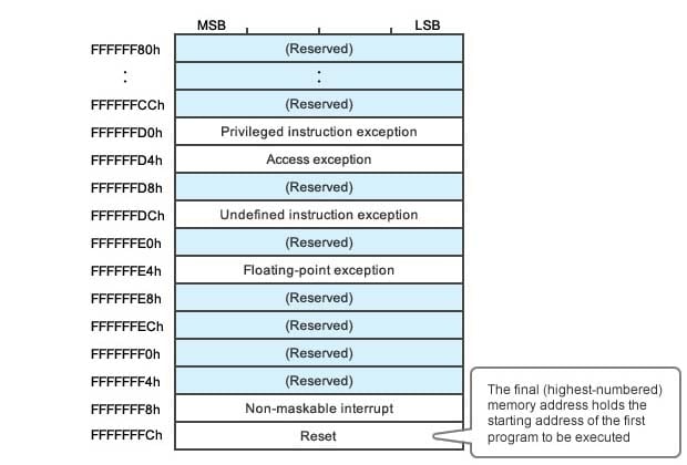
Figure 2. Vector Table Used by the RX63N Series
The RX63N uses a vector table. Since the address space is 32-bit, the vector table must hold a 4-byte value giving each start address (since all addresses are 32 bits long). As you can see in Figure 3, the very last four bytes of the memory space (FFFFFFCh to FFFFFFFh) hold the address at which the CPU will start execution following a reset. When a reset occurs, the CPU goes to these last four bytes, reads the address, and then jumps to that address and reads the first instruction.
Notice that the vector table includes other address values as well. These addresses, for example, tell the CPU where to go to start handling an exception (an anomalous or irregular event that requires suspension of normal program flow), and where to go when an interrupt occurs.
Let's consider how program execution proceeds when a vector table is in use. Figure 3 shows the processing that occurs when a non-maskable interrupt (NMI1) is thrown.
- The NMI occurs.
- The CPU reads the NMI handling address (in this example, 10000000h) from the NMI row of the vector table.
- The CPU reads and executes the instruction at 10000000h, which is the first instruction of the NMI handling routine.
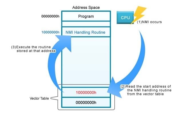
Figure 3: Vector Table Processing Flow
1. Non-Maskable Interrupt (NMI): An interrupt that cannot be disabled ("masked"). While the CPU can be set to ignore maskable interrupts, it must always respond to NMIs. Interrupts from watchdog timers, for example, are often non-maskable. (Watchdog timers were introduced here, in the second session of this series.)
One important benefit of using a vector table is that this approach makes it possible to freely arrange interrupt handlers in memory, since you can always use the table to tell the CPU where to go to find them.
To sum up: In this session, we have looked at CPU address space, at its relation to peripheral functions, and at where program execution begins following a reset or NMI. Note that CPU memory is a relatively costly resource and it is important to write compact code so as to conserve it; but, even so, a 32-bit MCU has a fairly large address space, and is much more flexible and less restrictive than 16-bit MCUs. This eliminates the need to perform all types of tricks to get the program code to fit, and makes it possible to arrange programs in memory in a manner that is easy for programmers and designers to understand and work with.
In the second part of this session, we will look at how processing and memory work together during program runtime, and at what this means with respect to writing efficient MCU programs.